Multimodal contrastive learning
This post introduces some basic concepts of contrastive learning to beginners. As its name suggests, contrastive learning is powered by contrasting the differences across instances (training samples) to learn a refined vector representation of data. This post focuses on one of the application scenarios, i.e., learning a shared embedding space across modalities, as popularized by CLIP from OpenAI\(^{[1]}\).
TL; DR
- Intuitive understanding of contrastive learning
- An often-used loss function -- infoNCE
- Applications of contrastive learning
- Some practical tips
Basic ideas behind contrastive learning
One fundamental problem in ML is to connect/associate data from different modalities, e.g., text and photo describing the same car, brain MRI scan and memory clinical test scores of the same patient. One way to achieve the association is to generate one from the other, for example predicting a sequence of words to describe an input image or generating a video that matches a voice recording. However, none of these are easy to achieve.
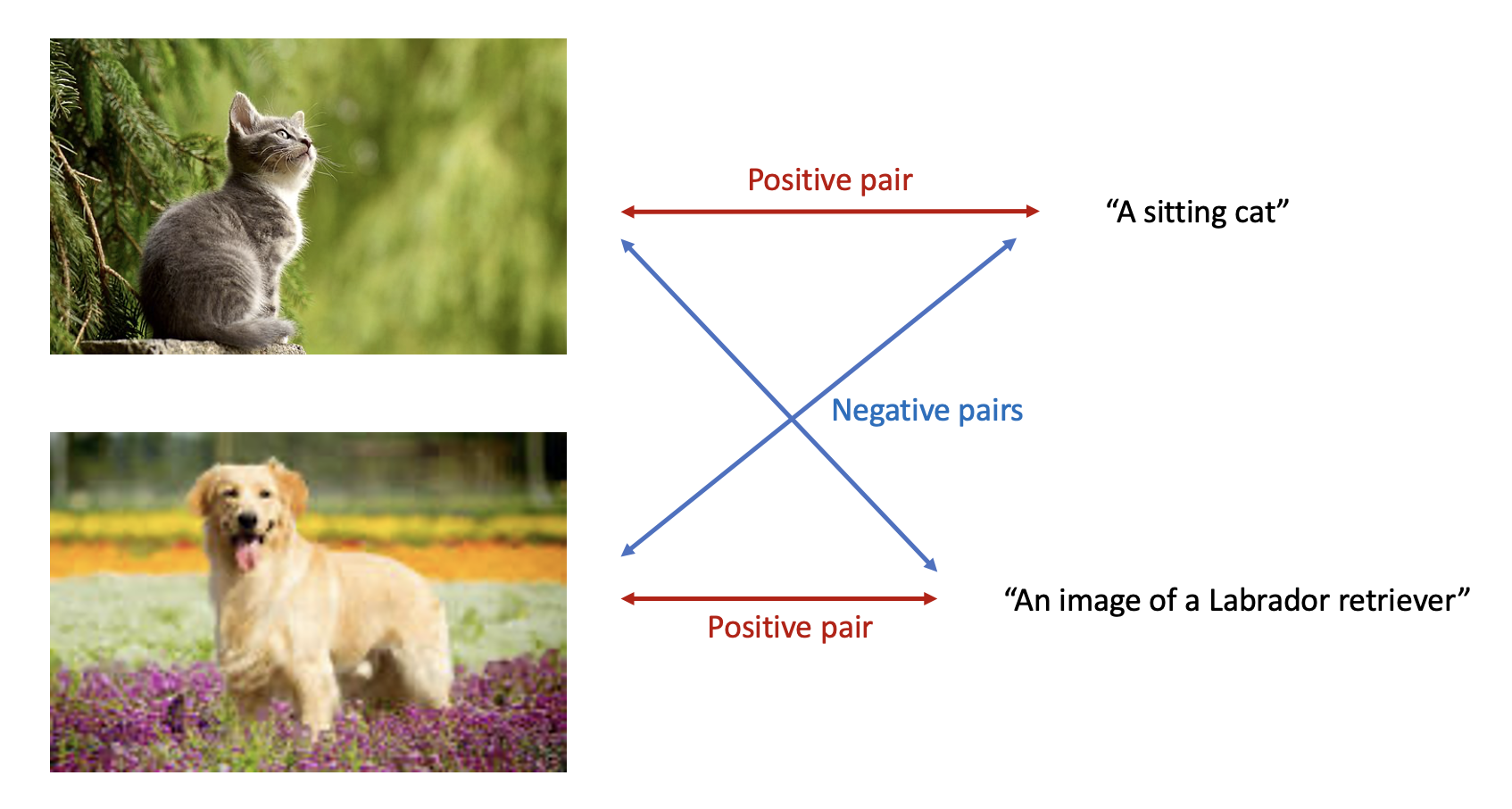
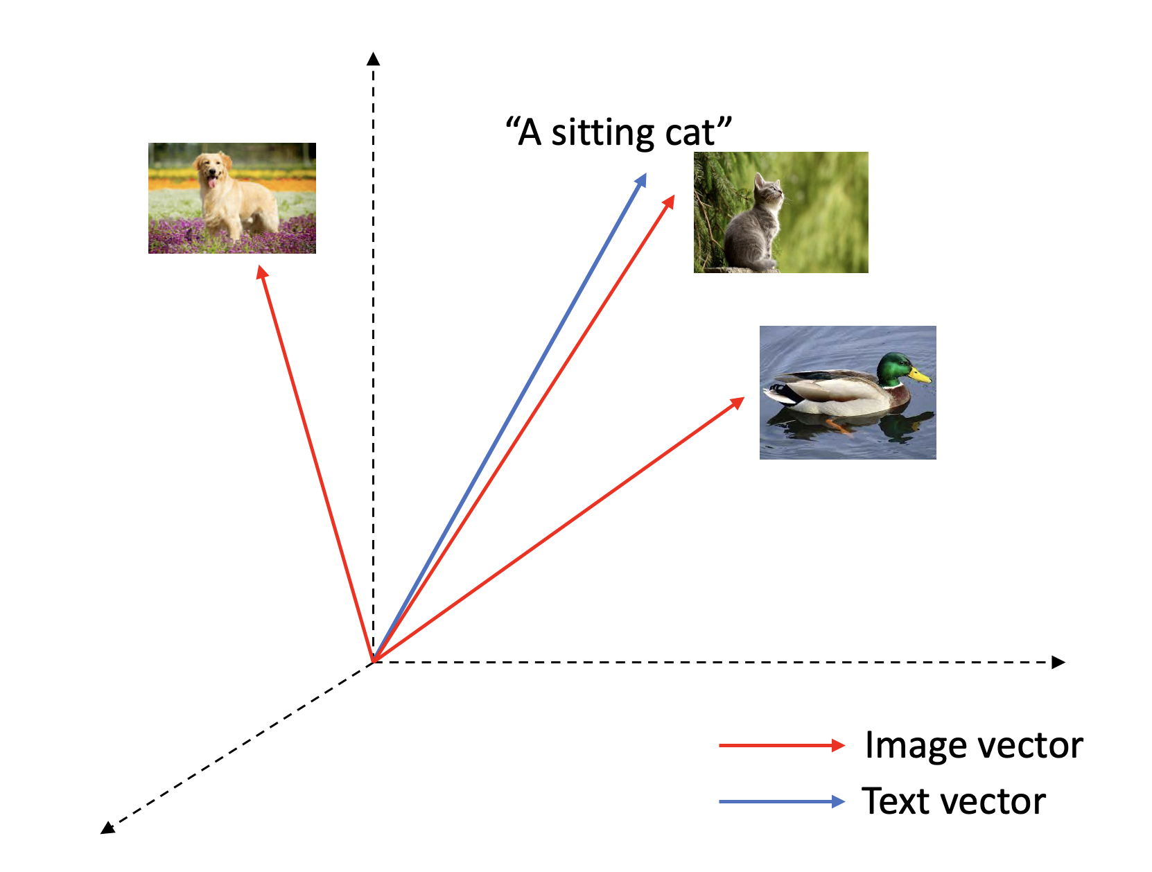
Contrastive learning offers an alternative way to build the cross-modality connection by mapping data (text, image, video, etc.) to a shared embedding space. An ideal embedding space satisfies the following properties: embedding vectors of data describing the same object (conventionally named as positive pairs) are close to each other, while embedding vectors of distinct objects (negative pairs) are not.

With an optimization strategy of pulling positive pairs closer and setting negative pairs apart, a meaningful embedding space should have been established in the end of training. You can then retrieve the most matching image to a query text or the most relevant description to an image from your data using cosine similarity between two vectors as a proxy for relevancy.

Loss function
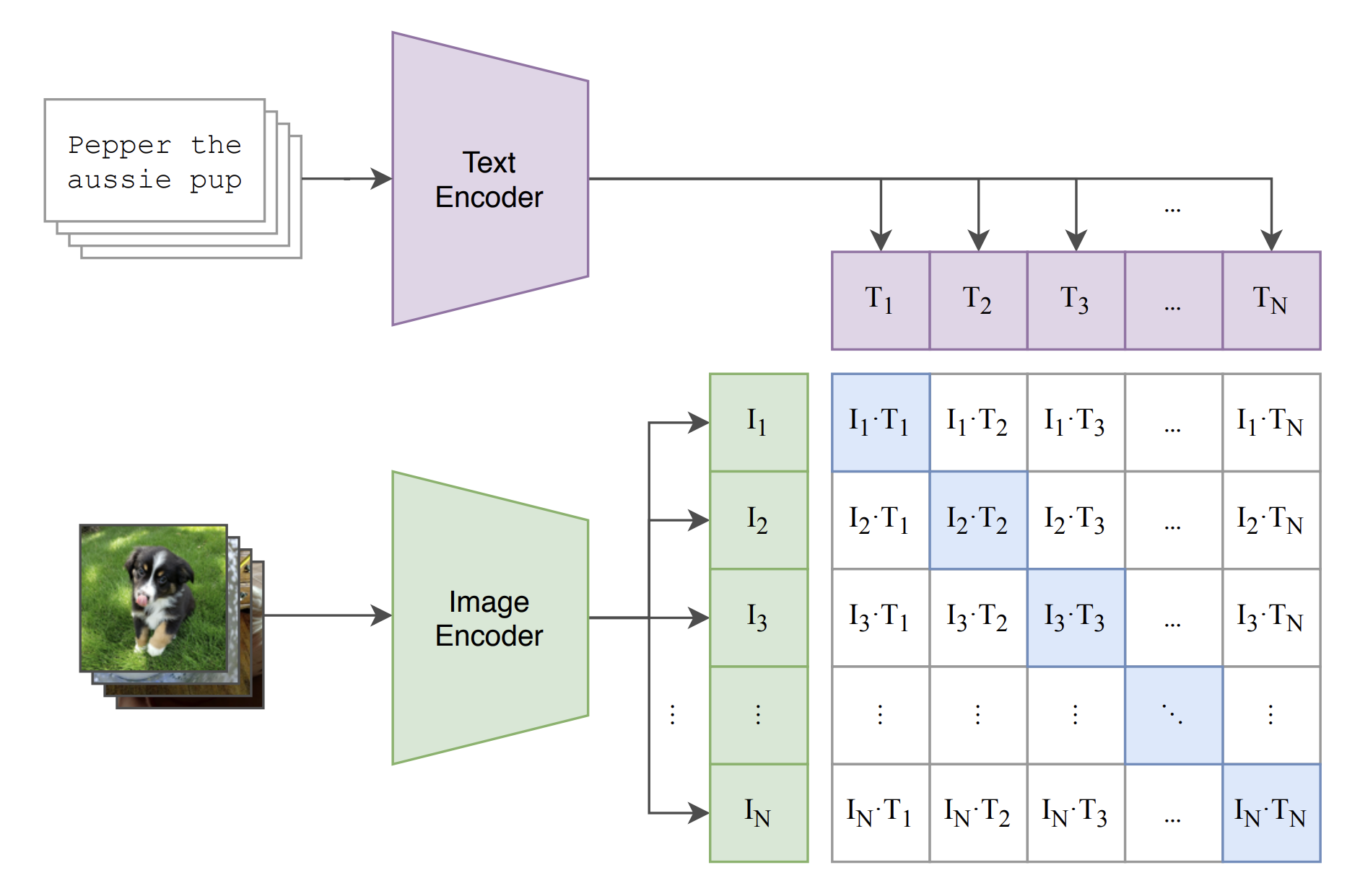
To understand the loss function used in the CLIP paper, it is helpful to have a picture of the problem formulation as illustrated in the schematics below. Text and imaging data are separately encoded into embedding vectors, where \(I_i\) represents the L2-normalized embedding vector of the \(i_{th}\) image, and \(T_j\) represents the L2-normalized embedding vector of the \(j_{th}\) text.
The similarity matrix \(M\), whose element value \(M_{ij} = I_{i} \cdot T_{j}\), characterizes the cosine similarity between any image-text pairs within a training batch. As only \(I_{i}\) and \(T_{i}\) form a positive pair, a sign of well-functioned embedding model is to yield large diagonal values and small off diagonal values in \(M\). To achieve this, one can train a multiclass classifier that optimizes the probability distribution in each row/column with the label equals \(i\) in the \(i_{th}\) row/column.

Thus, the loss function can simply be put as the sum of row-based and col-based cross-entropy loss as below.
\[L(I_{1}, ... ,I_{N}, T_{1}, ... T_{N}) = L_{row} + L_{col}\] \[L_{row} = -\sum_{i=1}^{N} log(\frac{exp(M_{ii})}{\sum_{j}exp(M_{ij})}), \space L_{col} = -\sum_{j=1}^{N} log(\frac{exp(M_{jj})}{\sum_{i}exp(M_{ij})})\]The loss function can also be viewed from the perspective of mutual information. Van den Oord, et al proofed in their InfoNCE paper\(^{[2]}\) that optimizing this loss actually maximizes the lower bound of mutual information between the embedding vectors \(I\) and \(T\).
Applications
Though the original CLIP paper is about connecting image to text, the applications of CLIP should be modality agnostic, allowing us to establish semantic associations between any two data modalities, such as image to sound, text to video, etc. It can also easily scale up to associate more data modalities by introducing extra terms in the loss function as below, where each term focuses on a pair of modalities.
\[loss = l(A, B) + l(A, C) + l(B, C)\]Assuming the encoder for each modality maps inputs to a cluster of points in a shared embedding space, the loss function pulls the clusters together and forms a nice mixture that the A, B, C vectors of the same instance are nearby to each other whereas vectors of distinct instances are not. Once the training part is done, these A, B, C vectors as a good representation of the instance can then be used for many down streaming tasks, like classification, segmentation, retrieval, etc.
To give a concrete example in the medical domain, researchers in the field of neurodegenerative diseases are interested in associating brain structural changes (captured by MRI scans) and functional deterioration (measured with scores from clinical assessments). Traditionally, people may create a multitask model with MRI as input to predict tens of or even hundreds of clinical scores in parallel outputs. The challenge of doing so is from strong interference among these prediction tasks, i.e., learning some tasks may distract the model from learning the others. With a setup of CLIP-based contrastive learning, we can establish a shared embedding space between MRI and clinical tests, and search for the best matching record of clinical measures to a target MRI from all existing clinical records or “new” records created from bootstrapping.
Similarly, if the goal is to predict brain structures given clinical measures, one may attempt to generate 3D high-resolution brain MRI scans from those numerical scores using frameworks like GAN (Generative Adversarial Network). However, it is technically challenging and computationally expensive to chase this direction. In addition to the concern of the generated image quality, a well-known issue of mode collapse may prevent the model from yielding a diverse output set. But with contrastive learning, one can retrieval the most matching MRI scan from all collected scans with even some image augmentations to increase the granularity of all MRI candidates.
Practical tips
Better to have large batch size
To fully harness the power of contrastive learning, it practically works better to use a large batch size during training. Since the model relies on the contrastive signals between the positive and negatives from a batch, having a large number of samples increases the chances of including more non-trivial negatives (i.e., those that share some similar concepts with the positive but still present differences from the positive that a good model would distinguish) and thus improve the embedding quality. Though training with huge batch size requires a good amount of GPU memory, one can always do some tricks to artificially increase the batch size, including (1) collecting embedding output from all GPUs to aggregate negatives from all GPUs, (2) creating a memory bank to cache negatives from previous iterations\(^{[3]}\).
Pay attention to the negatives
The performance of contrastive learning is all about how rich the negatives are. And we particularly are interested in the hard negatives and false negatives. Sometimes, the training data might be corrupted with false negatives (almost equivalent to the positive but labeled as negative) whose existence could greatly confuse the model. Thus, it is worth the effort to inspect if there are any false negatives and correct the labels accordingly. Mining hard negatives is also a hot direction to further improve the embedding quality especially when there is a strict limit on GPU resources. Better than blindly increasing batch size to hope for more negatives being sampled, people have designed clever ways\(^{[4]}\) to pick hard negatives to make force the model to learn more.
References
-
Radford, Alec, et al. “Learning transferable visual models from natural language supervision.” International Conference on Machine Learning. PMLR, 2021.
-
Oord, Aaron van den, Yazhe Li, and Oriol Vinyals. “Representation learning with contrastive predictive coding.” arXiv preprint arXiv:1807.03748 (2018).
-
He, Kaiming, et al. “Momentum contrast for unsupervised visual representation learning.” Proceedings of the IEEE/CVF conference on computer vision and pattern recognition. 2020.
-
Xiong, Lee, et al. “Approximate nearest neighbor negative contrastive learning for dense text retrieval.” arXiv preprint arXiv:2007.00808 (2020).
Enjoy Reading This Article?
Here are some more articles you might like to read next: